
Select menu: Stats | Distributions | Kernel Density Estimation
Use this to evaluate a Kernel density estimate for a selected variate. A Kernel Density estimate can be thought of as a smoothed form of a histogram.
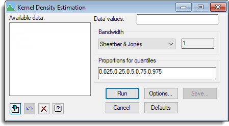
- After you have imported your data, from the menu select
Stats | Distributions | Kernel Density Estimation. - Fill in the fields as required then click Run.
You can set additional Options then after running, you can save the results by clicking Store.
Kernel density estimation is a useful tool for exploring the unknown underlying distribution of a sample. The kernel method constructs an estimate fh(t) of the true density function by placing a kernel function K(t;xi,h) over each observation xi in the sample. The kernel function K(t;x,h) is itself a density function with location parameter x and scale parameter h, also called bandwidth in this context. The density estimate is then given by
fh(t) = the sum of (K(t-xi)/h)/(nh) from i = 1...n
where n denotes the sample size. The choice of kernel function K is not very critical for the resulting estimate fh(t) and so a Gaussian kernel is used.
The following graph showing the sum of the normal kernels at 5 data points illustrates the ideas behind the kernel density estimation.

Bandwidth
The choice of bandwidth, h, is of crucial importance in kernel density estimation. A large value of h will give rise to an over smoothed density estimate, while a small value of h will produce a very ragged density with many spikes at the observations. It is recommended that a range of values of h be used, and the resulting kernel density estimates be examined, since this will highlight different features of the data.
For automatic use of kernel density estimation, estimation of the bandwidth h from the data is very helpful. The following automatic data driven estimates are available (n = the number of observations in the selected variate):
| Sheather & Jones | The method of Sheather & Jones (1991). Jones, Marron & Sheather (1996) recommend this for general purposes |
| Standard deviation | s1 = 1.06 * (standard deviation) * n**(-1/5) |
| Interquartile range | s2 = 0.79 * (inter quartile range) * n**(-1/5) |
| Min(Std Dev,IQ range) | s3 = 0.90 * minimum(standard deviation, interquartile range/1.34) * n**(-1/5) |
| Given | You provide your own estimate for the bandwidth in the associated field along side the dropdown list |
The s1,s2 and s3 estimates of bandwidth are popular due to their simplicity and are optimal in some sense for data from a normal distribution.
Proportions for quantiles
Proportions at which to calculate quantiles of the kernel density estimate. This is either a comma or space separated list of numbers or may be the name of an existing variate.
Action buttons
| Run | Process the Kernel Density Estimation on the selected data. |
| Options | Opens the Kernel Density Estimation Options dialog to allow various options to be set which control the output and graph. |
| Save | Open the Kernel Density Estimation Save Options dialog to specify save structures for the analysis. |
| Cancel | Close the dialog without running any more analyses. |
| Defaults | Reset all options to their default values. |
Action Icons
| Pin | Controls whether to keep the dialog open when you click Run. When the pin is down |
|
| Restore | Restore names into edit fields and default settings. | |
| Clear | Clear all fields and list boxes. | |
| Help | Open the Help topic for this dialog. |
See also
- Kernel Density Estimation Options
- Kernel Density Estimation Save Options
- KERNELDENSITY procedure in command mode
- Probability Distribution Plot
- Fit Distribution
- Further details of distributions
- Empirical Distribution Tests menu
- DISTRIBUTION directive in command mode